A common metric in the field of quantitative finance is the Sharpe ratio. The Sharpe ratio is a measure of the extent of the returns (over the risk-free rate) that a strategy will produce relative to the amount of risk it assumes. If a strategy has mean return $\mu$ and variance $\sigma^2$, and if the rate of return for a risk-free asset is $\mu^\star$, then the Sharpe ratio is simply the quantity, \begin{align} s = \frac{\mu - \mu^\star}{\sigma}. \end{align} Let’s see if we can gain some intuition for this quantity by considering a very simple game.

A Simple Game

Suppose we have a strategy that produces a one dollar return with probability $p$ but also has the possibility of losing one dollar with probability $1-p$. The question is, what is the Sharpe ratio of this game? To answer this, we will define a random variable for the profit on a given day, \begin{align} X = \begin{cases} +1 & \text{with probability } p \\
-1 & \text{with probability } 1-p \end{cases} \end{align} If there are 252 trading days in a year, the amount of money earned over a course of a year will be, \begin{align} S = X_1 + X_2 + \ldots + X_{252}, \end{align} where the $\left(X_i\right)_{i=1}^{252}$ are assumed to be independent. We need to analyze the expectation and variance of $S$. \begin{align} \mathbb{E}\left[S\right] &= \mathbb{E}\left[X_1\right] + \mathbb{E}\left[X_2\right] + \ldots + \mathbb{E}\left[X_{252}\right] \\
&= 252\mathbb{E}\left[X_1\right] \\
&= 252\left(2p - 1\right) \\
\mathbb{V}\left[S\right] &= \mathbb{V}\left[X_1\right] + \mathbb{V}\left[X_2\right] + \ldots + \mathbb{V}\left[X_{252}\right] \\
&= 252 \left(1 - \left(2p - 1\right)^2\right). \end{align}

Let’s assume a risk-free rate of zero. Therefore, the Sharpe ratio of this strategy is, \begin{align} s = \frac{252\left(2p - 1\right)}{\sqrt{252 \left(1 - \left(2p - 1\right)^2\right)}}. \end{align} Let’s plot the Sharpe ratio as a function of $p$. 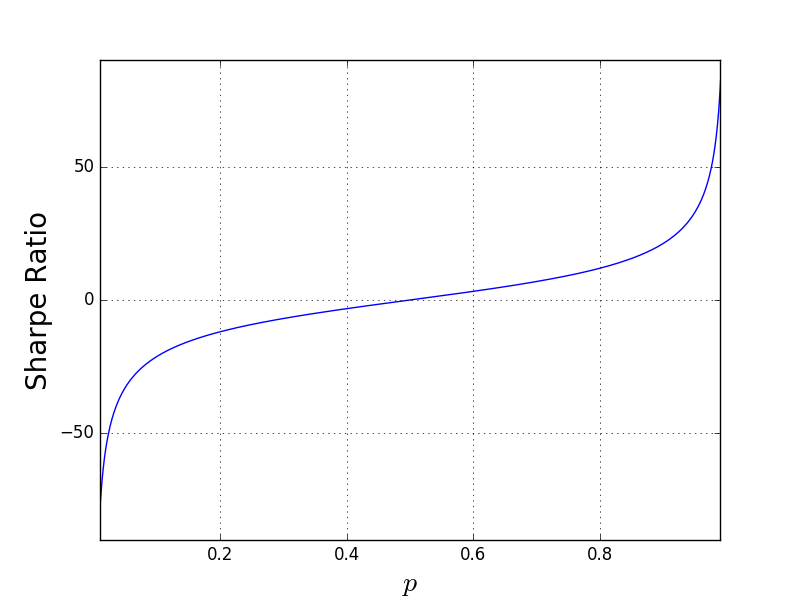Quite understandably, the Sharpe ratio is zero for $p=\frac{1}{2}$ and rapidly accelerates towards $\pm\infty$ as $p$ goes toward zero or one. What I find interesting about this plot is how small $p$ needs to be in order to realize a “high” Sharpe ratio. I think that most traders would agree that a Sharpe ratio of two is quite respectable, but in fact you only need $p \approx 0.563$ to achieve this. That’s only six percentage points higher than random guessing!

Python Code

Here’s some very simple Python code I used to check my answers and create the figure.

import numpy as np
import matplotlib.pyplot as plt


# Number of random trials.
n = 1000
# Probability of making a profit on any given day.
p = 0.8

# Create random profit-and-loss sequences.
X = (np.random.uniform(size=(252, n)) < p).astype(float)
X[X == 0.] = -1.
# Compute the expected profit at the end of the year.
S = X.sum(axis=0)

print("Empirical average:\t\t{}".format(S.mean()))
print("Theoretical average:\t{}".format(252 * (2*p - 1)))
print("Empirical variance:\t\t{}".format(S.var()))
print("Theoretical variance:\t{}".format(252 * (1 - (2*p - 1)**2)))

def sharpe(p):
    """Return the Sharpe ratio for a simple game."""
    return (252 * (2*p - 1)) / np.sqrt(252 * (1 - (2*p - 1)**2))


if True:
    p_range = np.linspace(0.0, 1., num=1000)
    plt.figure(figsize=(8, 6))
    plt.plot(p_range, sharpe(p_range))
    plt.xlabel("$p$", fontsize=20)
    plt.ylabel("Sharpe Ratio", fontsize=20)
    plt.grid()
    plt.xlim((0.01, 0.99))
    plt.ylim((-90, 90))
    plt.show()