Yesterday I was reading two very interesting papers, which basically express the same idea: That we can iteratively refine a variational posterior approximation by taking a Gaussian mixture distribution and appending components to it, at each stage reducing the KL-divergence between the true posterior and the mixture approximation. The two papers are Variational Boosting: Iteratively Refining Posterior Approximations and Boosting Variation Inference (you can see they almost have exactly the same name!). In this post, I want to try to connect at least one of the insights here to my research on Stein variational gradient descent.

Basically, a nice property about Gaussian mixture models is that they are very easy to sample from. In particular, if we form a Gaussian mixture via, \begin{align} p\left(x\right) = \frac{1}{k} \sum_{i=1}^{k} \omega_{i}\mathcal{N}\left(x; \mu_i, \sigma_i^2\right), \end{align} where $\left(\omega_i\right)_{i=1}^k$ sum to unity and represent positive mixture weights. It is easy to see that we can very quickly generate samples from the mixture. First we select a component of the mixture, and then we generate a random variate from that component. On the other hand, for Stein variational gradient descent (SVGD), it is not immediately clear to me how one can iteratively generate more and more observations from the unknown posterior. Because SVGD is a particle based method, it is most intuitively understood to be a mechanism for drawing a sample set of fixed size jointly. Compare this to a Markov chain Monte Carlo approach where you can run the chain ad infinitum to obtain an infinite number of samples.

What is there to be done about this? I can imagine situations where more posterior samples as desirable or required, but it would be an annoyance to have to re-sample using the SVGD algorithm from scratch. Moreover, it is known that the computational complexity of SVGD is quadratic in the number of samples to be drawn: For a fixed sample size of $n$, the computational burden to me is $\mathcal{O}\left(n^2\right)$. For large-scale inference, this isn’t going to work (although it still isn’t as bad as Gaussian processes!).

This got me thinking: If I’ve already sampled $n$ data points from my unknown posterior, how could I make it easier for myself to obtain the $n+1$th sample? One solution that I came up with drew inspiration from the variational boosting papers I mentioned before: Estimate a Gaussian mixture model based on the $n$ samples already collected, and then leverage the Gaussian mixture to yield further samples. For a relatively simple class of model (e.g. those with relatively small posterior dimensionality) I can see this working effectively. Using my library for Stein variational gradient descent, I implemented this strategy to see how it would work on a logistic regression task. Our first step is to generate some synthetic data.

import numpy as np

# Create synthetic logistic regression data.
n, k = 100, 2
X = np.random.normal(size=(n, k))
beta = np.ones((k, 1)) * 3
p = 1. / (1. + np.exp(-X.dot(beta)))
y = np.random.binomial(1, p)
# Create a test set.
n_test = 50
X_test = np.random.normal(size=(n_test, k))
p_test = 1. / (1. + np.exp(-X_test.dot(beta)))
y_test = np.random.binomial(1, p_test)

We can then define a logistic regression model in TensorFlow, where we impose a $\mathcal{N}\left(\mathbf{0}, \mathbf{I}\right)$ prior over the linear coefficients. Our log-posterior is then defined (up to an additive constant) by the log-likelihood and the logarithm of the normal prior probability.

import tensorflow as tf
from tensorflow.contrib.distributions import Normal

# Define a logistic regression model in TensorFlow.
with tf.variable_scope("model"):
    # Placeholders include features, labels, linear coefficients, and prior
    # covariance.
    model_X = tf.placeholder(tf.float32, shape=[None, k])
    model_y = tf.placeholder(tf.float32, shape=[None, 1])
    model_w = tf.Variable(tf.zeros([k, 1]))
    # Compute prior.
    with tf.variable_scope("priors"):
        w_prior = Normal(tf.zeros([k, 1]), 1.)
    # Compute the likelihood function.
    with tf.variable_scope("likelihood"):
        logits = tf.matmul(model_X, model_w)
        log_l = -tf.reduce_sum(tf.nn.sigmoid_cross_entropy_with_logits(
            labels=model_y, logits=logits
        ))
    # Compute the log-posterior of the model.
    log_p = (
        log_l +
        tf.reduce_sum(w_prior.log_prob(model_w))
    )

Now we can use Stein to sample from the posterior distribution over linear coefficients as follows:

from stein.samplers import SteinSampler
from stein.gradient_descent import AdamGradientDescent


# Number of particles.
n_particles = 200
# Number of learning iterations.
n_iters = 100
n_prog = n_iters // 10
# Sample from the posterior using Stein variational gradient descent.
gd = AdamGradientDescent(learning_rate=1e-1)
sampler = SteinSampler(n_particles, log_p, gd)

# Perform learning iterations.
for i in range(n_iters):
    if i % n_prog == 0:
        print("Progress: {} / {}".format(i, n_iters))
    sampler.train_on_batch({model_X: X, model_y: y})

At this point we have collected two-hundred two-dimensional particles representing a draw from the posterior distribution of our logistic regression model. In this case, with only two posterior dimensions, it does not seem unreasonable to fit a Gaussian mixture distribution to this data and leverage that for further sampling purposes; this would certainly be faster than relying on SVGD for all our sampling needs. To achieve this, I will use a variational Gaussian mixture model. Such models have two principal advantages (which I restate from their documentation here):

1. Automatic determination of the number of clusters in the dataset. This is achieved by formulating a variational Gaussian mixture with an upper limit on the number of possible clusters; then, during learning, certain clusters will have their contribution crushed to zero, thereby allowing only meaningful clusters to take effect. This contrasts to Gaussian mixture models learned through expectation propagation (EP), in which all components of the mixture tend to be used.
2. As a fundamentally Bayesian method, variational Gaussian mixtures have built-in regularization. Unlike variational Gaussian mixtures, those learned with EP can occasionally learn degenerate solutions that drive the likelihood to near infinity.

Fortunately, it is not necessary for us to implement the variational Gaussian mixture ourselves, since it is already implemented in the scikit-learn package for Python. In order to evaluate the efficacy of the learned Gaussian mixture, I propose to keep a holdout set of particles learned via SVGD and compute the log-likelihood of these particles under the estimated variational Gaussian mixture model. When the log-likelihood is high, it indicates that the generative ability of the mixture distribution is good. (It is clear from the above diagram that I would not need twenty-five mixture components, but I set it to an unreasonably high value to set robustness to misspecification.)

from sklearn.mixture import BayesianGaussianMixture


# Extract samples from Stein variational gradient descent.
theta = sampler.samples
n_test = int(n_particles * 0.9)
theta_train, theta_test = theta[:n_test], theta[n_test:]
# Cluster them.
m = BayesianGaussianMixture(
    n_components=25,
    n_init=1,
    weight_concentration_prior=1e-7,
    mean_precision_prior=1e-7,
    weight_concentration_prior_type="dirichlet_process",
).fit(theta_train)
ll_train = m.score_samples(theta_train).mean()
ll_test = m.score_samples(theta_test).mean()
# Show diagnostics.
print(
    "Train set log-likelihood: {:.4f}. "
    "Test set log-likelihood: {:.4f}".format(ll_train, ll_test)
)

This code yields the following output.

Train set log-likelihood: -1.0835. Test set log-likelihood: -1.1704

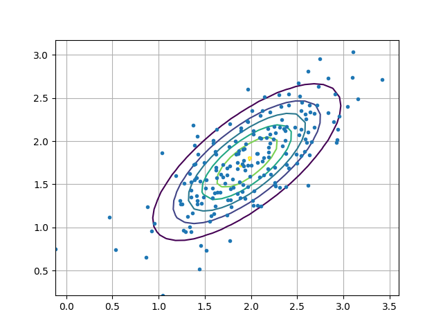
Now we can evaluate the efficacy of our posterior by comparing samples obtained directly from SVGD with samples drawn from the Gaussian mixture. We also visualize the posterior as follows, along with the Gaussian mixture approximation.

# Now evaluate the likelihood of sampled points.
n_samples = 500
beta_hat = m.sample(n_samples=n_samples)[0]

def accuracy(beta):
    """Computes the average accuracy on the test set for a set of posterior
    linear coefficients.
    """
    p_hat = 1. / (1. + np.exp(-X_test.dot(beta.T)))
    y_hat = (p_hat > 0.5) * 1.
    # Initialize a vector to store the accuracy for each set of linear
    # coefficients.
    acc = np.zeros((beta.shape[0], ))
    for i in range(beta.shape[0]):
        acc[i] = np.mean(y_hat[:, i] == y_test.ravel())
    # Return the average accuracy.
    return acc

# Show diagnostics.
acc_gm = accuracy(beta_hat)
acc_sg = accuracy(theta)
print("Gaussian mixture: {} / {}".format(
    acc_gm.mean(), acc_gm.std())
)
print("True posterior: {} / {}".format(acc_sg.mean(), acc_sg.std()))

This produces an estimate of the mean and variance of the accuracy for both the samples drawn using SVGD and samples from the Gaussian mixture model: The average accuracy under the true posterior is 78.36% and under the approximation it is 78.44%; the standard deviation of the accuracy under the true posterior is 0.02027 and under the approximation it is 0.01974. This demonstrates that the Gaussian mixture has properly captured the first two modes of the accuracy when SVGD is used to represent the truth. As further work in this direction, I’d like to assess ways that this could be leveraged in a practical application (in something less trivial than synthetic logistic regression). There’s also some intriguing phenomenons regarding Gaussian mixture modeling that further demonstrate the usefulness of variational modeling that I’ll discuss in a later post.