In our last discussion, we focused on the kernelized Stein discrepancy and how variational Stein gradient descent can be leveraged to sample from posterior distributions of Bayesian models. Our application area in that case was specifically Bayesian linear regression, where a prior (with a fixed precision) was placed over the linear coefficients of the linear model. Unfortunately, Bayesian linear regression is somewhat uninteresting because it is possible to compute the closed-form posterior for the coefficients. In this post, we’ll demonstrate two statistical models where this is not the case: logistic regression and Bayesian neural networks.

Modularizing Stein Variational Gradient Descent

Before continuing, I wanted to discuss some of the software engineering considerations I made while writing this blog post. In particular, I decided to try to write a set of class objects for performing Stein variational gradient descent for a specified log-posterior distribution. The purpose of this software, which I’ve named Stein, is to provide an easy-to-use framework for performing Bayesian inference with Stein variational gradient descent.

Stein is very much still a work-in-progress and there is much that can still be done in terms of abstracting away complexity and advancing utility. Nonetheless, I wanted to show off what Stein can do in its current state. Therefore, I’ve chosen to archive the current state of the project on GitHub which will provide a working implementation of the examples in this post even as the project continues to evolve. Please check it out and feel free to contribute!

For future directions, I would like to expand this library to include a declarative interface for specifying the target distribution, very similar to what Dustin Tran has accomplished with the Edward library. I’m also interested in replicating the research that has been conducted on reinforcement learning and GANs with Stein variational gradient descent. Finally, I wish to eventually port Stein from using Theano to using Tensorflow.

Logistic Regression

We’ll begin with the case of logistic regression. Throughout this post, I’ll be drawing extensively from the experiments of Dilin Wang and Qiang Liu in the original NIPS paper on Stein variational gradient descent. For logistic regression, they choose to examine a dataset of forestry cover types, consisting of 581,012 example data points and 54 explanatory features. Because the dataset is so large, it is not feasible to estimate a logistic regression model using a second-order method such as Fisher scoring; instead, a first-order gradient descent procedure must be used. Formally, the Bayesian model for logistic regression can be expressed as follows, \begin{align} y \vert \mathbf{X}, \boldsymbol{\beta} &\sim \text{Bern}\left(\sigma\left(\mathbf{X}’\boldsymbol{\beta}\right)\right) \\
\boldsymbol{\beta} &\sim \mathcal{N}\left(\mathbf{0}, \alpha^{-1}\mathbf{I}\right) \\
\alpha &\sim \text{Gamma}\left(a_0, b_0\right), \end{align} where $\sigma\left(x\right) = \frac{1}{1 + \exp\left(-x\right)}$ and $a_0$ and $b_0$ are Bayesian model hyperparameters. The posterior distribution, therefore, can be expressed proportionally to the likelihood and the priors, \begin{align} p\left(\boldsymbol{\beta}, \alpha \vert \mathbf{y}, \mathbf{X}\right) \propto \prod_{i=1}^{n} p\left(y_i \vert \mathbf{X}_i, \boldsymbol{\beta}\right) p\left(\boldsymbol{\beta}\vert\alpha\right) p\left(\alpha\right). \end{align} Sampling from this distribution is usually achieved by Markov chain Monte Carlo, but that is not the approach we will adopt here.

As a practical matter, it is important to note that $\alpha$ is constrained to be positive since it is a precision parameter. However, there is no guarantee in gradient descent that a subsequent step will not result in a negative value of $\alpha$. As a result, we instead update $\log\alpha$ and exponentiate that value to obtain the precision over the linear coefficients. Therefore, let $\gamma = \log\alpha$. We can derive the gradient of the log-posterior distribution as follows, \begin{align} \nabla_{\boldsymbol{\beta}} p\left(\boldsymbol{\beta}, \alpha \vert \mathbf{y}, \mathbf{X}\right) &= \left(\mathbf{y} - \sigma\left(\mathbf{X}\boldsymbol{\beta}\right)\right)’\mathbf{X} - \alpha \boldsymbol{\beta} \\
\nabla_{\gamma} p\left(\boldsymbol{\beta}, \alpha \vert \mathbf{y}, \mathbf{X}\right) &= \frac{k}{2} - \frac{\alpha}{2} \boldsymbol{\beta}’\boldsymbol{\beta} - \frac{\alpha}{100} + 1, \end{align} where we have leveraged the fact that in our experiments $a_0=1$ and $b_0=1/100$ and $\mathbf{X}\in \mathbb{R}^{n\times k}$.

In our experimental setup, we seek to replicate the parameters of Qiang and Liu. Specifically, we use twenty percent of the forestry covertype data as a test set (selected at random), we use minibatches of fifty randomly selected samples, we use one-hundred particles to sample from the posterior, we set $a_0=1$ and $b_0=1/10$, and we use a learning rate of $1/100$. The forestry covertype data can be downloaded from here. Lastly, we note that in the forestry covertype dataset the target variable is rescaled to $\left\{-1, +1\right\}$, which changes some of the mathematics from the usual binary class logistic regression formulation. Now I’ll demonstrate how Stein can be leveraged to sample from the posterior of a Bayesian logistic regression model.

For simplicity, I’ll split up the disparate components of the Bayesian logistic regression main.py and discuss each individually. To begin with, we’ll simply load the forestry covertype data.

# File: main.py
import numpy as np
from scipy import io
from sklearn.model_selection import train_test_split

# For reproducibility.
np.random.seed(0)

# Load data and partition into training and testing sets.
data = io.loadmat("./data/covertype.mat")["covtype"]
data_X, data_y = data[:, 1:], data[:, 0]
data_y[data_y == 2] = -1
X_train, X_test, y_train, y_test = train_test_split(
    data_X, data_y, test_size=0.2, random_state=0
)

# Size of minibatches during training.
n_batch = 50
# Number of training data points.
n_train = X_train.shape[0]

Next, we provide Python code for computing the gradient of the log-posterior distribution over the linear coefficients and precision over those coefficients. It is important to note that because we are training the logistic regression model using minibatches, we need to rescale the likelihood component of the posterior by the ratio $n / n_{\text{batch}}$.

# File: main.py
def grad_log_p(theta):
    """Gradient of the Bayesian logistic regression posterior distribution with
    respect to the linear coefficients as well as the precision over the
    coefficients.
    """
    # Select a minibatch on which to compute the gradient.
    batch_idx = np.random.choice(n_train, n_batch)
    X, y = X_train[batch_idx], y_train[batch_idx]
    # Extract logistic regression parameters.
    w = theta[:-1]
    alpha = np.exp(theta[-1])
    d = len(w)
    # Compute the linear component of logistic regression and compute the
    # probability of class one.
    linear = X.dot(w)
    p_hat = 1.0 / (1.0 + np.exp(-linear))
    # Gradient of the likelihood with respect to the coefficients.
    dw_data = ((y + 1.) / 2.0 - p_hat).T.dot(X)
    # Gradient of the prior over coefficients.
    dw_prior = -alpha * w
    # Rescale gradient.
    dw = dw_data * X_train.shape[0] / X.shape[0] + dw_prior
    # Notice that we are performing gradient descent on the logarithm of the
    # prior precision. That's why this gradient is slightly different.
    dalpha = d / 2.0 - (alpha / 2.) * w.dot(w) - 0.01 * alpha + 1.

    return np.append(dw, dalpha)

To evaluate the logistic regression model, we will consider the out-of-sample accuracy. Because we have multiple samples from the posterior, we average over the class-one probabilities before thresholding against $1/2$.

# File: main.py
def evaluation(theta, X_test, y_test):
    """Compute the test set accuracy of the Bayesian logistic regression
    algorithm using the posterior samples of the linear coefficients. Notice
    that we average class one probabilities over each particle before
    thresholding against one-half.
    """
    # Disregard the posterior precision over the linear coefficients.
    theta = theta[:, :-1]
    # Extract the number of particles and the number of testing data points.
    M = theta.shape[0]
    n_test = X_test.shape[0]
    # Compute the predictions from the Bayesian neural network.
    p_hat = 1. / (1. + np.exp(-X_test.dot(theta.T)))
    y_hat = (p_hat.mean(axis=1) > 0.5) * 2. - 1.

    return np.mean(y_hat == y_test)

# Create a function to serve as an evaluator in the Stein sampler class.
evaluator = partial(evaluation, X_test=X_test, y_test=y_test)

At this stage, all of the necessary components for training a Bayesian logistic regeression model with Stein variational gradient descent are in place. To sample from the posterior, we only need the following code,

# File: main.py
# Setup parameters of the Stein sampler.
n_particles = 100
n_params = X_train.shape[1] + 1
n_iters = 6000
# Specify that the Stein sampler should use a squared exponential kernel.
kernel = SquaredExponentialKernel(n_params)
# Create a gradient descent object for Stein variational gradient descent.
gd = Adagrad(learning_rate=1e-2)

# Create the Stein sampler.
stein = SteinSampler(grad_log_p, kernel, gd, evaluator=evaluator)
# Sample using Stein variational gradient descent with a squared exponential
# kernel on the posterior distribution over the parameters of a Bayesian
# logistic regression model.
theta = stein.sample(n_particles, n_iters)

# Compute the test set performance of the algorithm.
acc = evaluation(theta, X_test, y_test)
print("Accuracy:\t{}".format(acc))

Running this code obtains an out-of-sample accuracy of 75.677%, which appears to be competitive with the results reported by Qiang and Liu.

Bayesian Neural Networks

There has been a lot of recent interest in developing neural networks with well-calibrated uncertainties. For a good reference on this area, I suggest heading on over to Yarin Gal’s blog. The essential idea behind Bayesian neural networks is that we can place priors over the weights and biases of the network and derive a posterior distribution of weights and biases given observed data; this allows us to sample neural network parameters that explain the data well, but yield varying outputs on unseen data. This permits us to capture uncertainty in neural networks, which can be important for decision-making pipelines, adversarial learning, and other domains.

The mathematical model for a basic Bayesian neural network can be defined as follows, \begin{align} p(\mathbf{y} \vert \mathbf{W}, \mathbf{X}, \gamma) &= \prod_i^{n} \mathcal{N}\left(y_i \vert \text{NN}\left(\mathbf{X}_i; \mathbf{W}\right), \gamma^{-1}\right) \\
p(\mathbf{W} \vert \lambda) &= \mathcal{N}\left(\mathbf{W} \vert \mathbf{0}, \lambda^{-1}\mathbf{I}\right) \\
p(\gamma) &= \text{Gamma}\left(\gamma \vert \alpha, \beta\right) \\
p(\lambda) &= \text{Gamma}\left(\lambda | \alpha, \beta\right), \end{align} where $\text{NN}\left(\mathbf{x};\mathbf{W}\right)$ is a neural network as follows, \begin{align} \text{NN}\left(\mathbf{X}_i;\mathbf{W}\right) = \text{RELU}\left(\mathbf{X}_i\mathbf{W}_1 + \mathbf{b}_1\right)\mathbf{W}_2 + b_2; \end{align} that is, a single-layer neural network with a scalar output and a RELU activation function: $\text{RELU}\left(x\right) = \max\left\{0, x\right\}$.

Before we apply our Bayesian neural network infrastructure to predicting Boston housing prices (a common test dataset), it is useful to consider the following toy example: Suppose we are interested in modeling a random variable of the form $y\sim\mathcal{N}\left(\sin 5x, \frac{1}{100}\right)$. If we observe a sample of fifty points, let us assume that we have a mechanism for sampling from the posterior distribution of weights and biases; then, because this is a simple one-dimensional regression problem, we can sample functions from the posterior distribution of neural networks and overlay them to characterize the uncertainty in the predictions. In the figure below, I’ve plotted fifty samples from this posterior alongside the training data and true underlying signal. 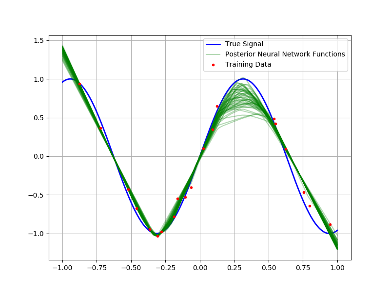Notice how the different functions correspond to varying interpretations of the underlying data. Most of the draws explain the underlying data quite well, the variation in out-of-sample regions reflects the model’s uncertainty about the behavior of the underlying function. One also notices the abrupt changes in directionality of the interpolation; this is due to the RELU nonlinearity.

For demonstrating how to implement sampling from Bayesian neural networks with Stein I will not post the entire code (for that, please see here). However, I would like to point out that I utilize the automatic differentiation capabilities of Theano for computing the gradient of the log-posterior distribution. This is very convenient and unlikely to result in the mistakes of deriving the gradient by hand.

# File: construct_neural_network.py
import numpy as np
import theano.tensor as T
import theano


def construct_neural_network(n_params, alpha, beta, nonlin=T.nnet.relu):
    # Data variables.
    X = T.matrix("X") # Feature matrix.
    y = T.vector("y") # Labels.
    # Network parameters.
    w_1 = T.matrix("w_1") # Weights between input layer and hidden layer.
    b_1 = T.vector("b_1") # Bias vector of hidden layer.
    w_2 = T.vector("w_2") # Weights between hidden layer and output layer.
    b_2 = T.scalar("b_2") # Bias of output.
    # Number of observations.
    N = T.scalar("N")
    # Variances parameters.
    log_gamma = T.scalar("log_gamma")
    log_lambda = T.scalar("log_lambda")

    # Prediction produced by the neural network.
    prediction = T.dot(nonlin(T.dot(X, w_1) + b_1), w_2) + b_2
    # Define the components of the log-posterior distribution.
    log_likelihood = (
        -0.5 * X.shape[0] * (T.log(2*np.pi) - log_gamma)
        - (T.exp(log_gamma)/2) * T.sum(T.power(prediction - y, 2))
    )
    log_prior_data = (
        (alpha - 1.) * log_gamma - beta * T.exp(log_gamma) + log_gamma
    )
    log_prior_w = (
        -0.5 * (n_params-2) * (T.log(2*np.pi)-log_lambda)
        - (T.exp(log_lambda)/2)*(
            (w_1**2).sum() + (w_2**2).sum() + (b_1**2).sum() + b_2**2
        ) + (alpha - 1.) * log_lambda - beta * T.exp(log_lambda) + log_lambda
    )

    # Rescaled log-posterior because we're using minibatches.
    log_posterior = (
        log_likelihood * N / X.shape[0] + log_prior_data + log_prior_w
    )
    dw_1, db_1, dw_2, db_2, d_log_gamma, d_log_lambda = T.grad(
        log_posterior, [w_1, b_1, w_2, b_2, log_gamma, log_lambda]
    )

    # Compute the prediction of the neural network.
    prediction_func = theano.function(
        inputs=[X, w_1, b_1, w_2, b_2], outputs=prediction
    )
    # Compute the gradient.
    grad_log_p_func = theano.function(
        inputs=[X, y, w_1, b_1, w_2, b_2, log_gamma, log_lambda, N],
        outputs=[dw_1, db_1, dw_2, db_2, d_log_gamma, d_log_lambda]
    )

    return prediction_func, grad_log_p_func

Automatic differentiation libraries such as Theano and Tensorflow make use Stein very easy from an implementation perspective. (My intention is for this to only get easier with time.)

There are several tricks that are being used in applying a Bayesian neural network to the Boston housing dataset.

1. The training data is scaled to have mean zero and unit variance; these scaling factors are computed on the training set and then applied to the data in the test set to avoid introducing bias.
2. The $\gamma$ parameter, which is the noise precision of the model, is fine-tuned using a development set; this allows for increased likelihood of predictions under the posterior distribution and avoids introducing very small noise variance parameters. The development set is taken as a random subset of the training data.

The results of training the Bayesian neural network are summarized in the following table for a few chosen iterations of Stein variational gradient descent. By the ten-thousandth iteration, $\gamma$ selection on the development set has occurred, which drastically improves the out-of-sample log-likelihood.

Number of Iterations	0	1,000	2,000	5,000	8,000	10,000
Log-Likelihood	-8.0652	-7.2431	-7.8543	-32.2579	-27.9155	-2.5591
Root Mean Squared Error	9.9902	3.3338	2.6738	2.3447	2.3313	2.32600

The performance at 2,000 iterations looks to be comparable with the average performance stated by Qiang and Wang, and root mean squared error continues to improve after that point.

Future Directions

As I continue to write this series I will keep you updated on progress I make with the Stein library for Stein variational gradient descent. I would immediately like to look for applications of the methodology to interesting areas such as generative and reinforcement learning.

Copyright Disclaimer

I am grateful to Qiang Liu and Dilin Wang for their open-source implementation of Stein variational gradient descent. Since I have borrowed and adapted aspects of their code for this post, in accordance with the terms of their license, their copyright is preserved below.

© Qiang Liu and Dilin Wang 2016