Stein variational gradient descent is a technique developed by the Dartmouth machine learning group. The essential idea to perturb samples from a simple distribution until they approximate draws from a target distribution. This method relies crucially on Stein’s identity, which states, the following: \begin{align} \mathbb{E}_{x \sim p(x)}\left[\mathcal{A}_p\phi\left(x\right)\right] &= 0 \\
\mathcal{A}_p\phi\left(x\right) &= \phi\left(x\right)\nabla_x \log p(x)’ + \nabla_x \phi\left(x\right). \end{align}

An Example of Stein’s Identity

It will be illustrative to look at a particular example of Stein’s identity. Let $X$ be a standard normal random variable. Then we have, \begin{align} \log p(x) &= -\frac{1}{2} \log 2\pi - \frac{x^2}{2} \\
\nabla_x \log p(x) &= -x \end{align} Then, if $\phi\left(x\right) = x^3$, we obtain, \begin{align} \mathbb{E}\left[\mathcal{A}_p\left(x\right)\right] &= \mathbb{E}\left[x^2 \cdot -x\right] + 2\mathbb{E}\left[x\right] \\
&= -\mathbb{E}\left[x^3\right] + 2\mathbb{E}\left[x\right] \\
&= 0, \end{align} as claimed.

Stein’s Identity as a Discrepancy Measure

Generally speaking, if we instead consider the expectation, $\mathbb{E}_{x\sim q}\left[\mathcal{A}_p \phi(x)\right]$ then this will not be equal to zero for general $\phi$, where $q$ is some distribution with the same support as $p$. This gives rise to the idea that we can measure the difference between probability distributions by considering the degree of violation of Stein’s identity. In particular, the Stein discrepancy is defined to be, \begin{align} \mathbb{S}\left(q,p\right) = \max \left(\mathbb{E}_q\left[\text{tr}\left(\mathcal{A}_p \phi(x)\right)\right]^2 : \phi\in\mathcal{F}\right), \end{align} where $\mathcal{F}$ is a predetermined set of functions.

The Dartmouth machine learning group made the important observation that when $\mathcal{F}$ is chosen to be a reproducing kernel Hilbert space (RKHS) with kernel $k\left(\cdot,\cdot\right)$ with functions restricted to have unit norm under the RHKS, the $\phi\in\mathcal{F}$ that results in the greatest Stein discrepancy can be found in closed-form. In particular, \begin{align} \phi^\star(y) \propto \mathbb{E}_{x\sim q}\left[\mathcal{A}_p k(x, y)\right] \end{align} This furthermore facilitates a fascinating connection between the greatest violation of Stein’s identity and gradient descent on a KL-divergence. This result can be stated as follows:

Theorem (Stein Variational Gradient Descent)

Let $p(x)$ and $q(x)$ be densities and let $x\sim q(x)$. Consider the smooth transform $z = T(x) = x + \epsilon \phi(x)$ for a smooth vector function $\phi$. Denote by $q_T(x)$ the density of $z$ when $x$ is drawn from $q$. Then, the following relationship holds: \begin{align} \nabla_{\epsilon} \text{KL}\left(q_T || p\right) \bigg|_{\epsilon=0} = -\mathbb{E}_q\left[\text{tr}\left(\mathcal{A}_p\phi(x)\right)\right]. \end{align} This presents the question: How should one select $\phi(x)$ in order to maximally decrease the KL-divergence by perturbing $x$ in that direction? Using the previous result, where $\phi$ are chosen to be in a RKHS of bounded norm, it is clear that the perturbation direction presenting the maximal decrease is given again by, \begin{align} \phi^\star(y) \propto \mathbb{E}_q\left[\mathcal{A}_p k(x, y)\right]. \end{align} Hence, when $T(x) = x + \epsilon \phi^\star(x)$, \begin{align} \nabla_{\epsilon} \text{KL}\left(q_T || p\right) \bigg|_{\epsilon=0} = -\sqrt{\mathbb{S}\left(q, p\right)} \end{align}

Demonstration of the Theorem

Let the target distribution be $\mathcal{N}\left(0, \sigma^2\right)$ and let $x\sim \mathcal{N}\left(0,1\right)$. We will use the smooth transform given by the identity: $\phi(x) = x$; clearly, if $z = T(x) = x + \epsilon x$ then $z \sim \mathcal{N}\left(0, (1+\epsilon)^2\right)$. We will proceed first by computing the KL-divergence between $\mathcal{N}\left(0, (1+\epsilon)^2\right)$ and $\mathcal{N}\left(0, \sigma^2\right)$ and then compare that value to the (negative) of the violation of Stein’s identity for this $\phi$. To point: \begin{align} \text{KL}\left(q_T \vert\vert p\right) = \log\frac{\sigma}{1+\epsilon} + \frac{\left(1+\epsilon\right)^2}{2\sigma^2} - \frac{1}{2} \end{align} and differentiating, \begin{align} \frac{\partial \text{KL}}{\partial\epsilon}\bigg|_{\epsilon=0} = \frac{1+\epsilon}{\sigma^2} - \frac{1}{1+\epsilon}\bigg|_{\epsilon=0} = \frac{1}{\sigma^2} - 1 \end{align}

To verify, we now compute the violation of Stein’s identity. First, note that $\nabla_x \log p(x) = - \frac{x}{\sigma^2}$. Therefore, \begin{align} \mathbb{E}_{q}\left[\mathcal{A}_{p}x\right] &= \mathbb{E}_{q}\left[-\frac{x^2}{\sigma^2} + 1\right] \\
&= -\frac{1}{\sigma^2} + 1, \end{align} which, after taking the negative, is exactly the gradient of the KL-divergence.

Rather than considering just a single step of the Stein variational gradient descent process, we’ll continue this example to construct a sequence of distributions leveraging the theorem. In particular, viewing the tranformation $T(x) = x\left(1+\epsilon\right)$ as an $\epsilon$-perturbation in the variance of $x$, we can move $q_T$ toward the target distribution $p(x)$. In the following code, we have initialized $q$ to be $\mathcal{N}\left(0, 1\right)$ and have assigned a target distribution of $\mathcal{N}\left(0, 0.1\right)$; we perform 200 learning iterations with a learning rate of 0.01.

import numpy as np
from scipy import stats


def kl_divergence(lambda_sq, sigma_sq):
    """Compute the KL-divergence between two normal distributions with mean zero
    and distinct variances.

    Parameters
    ----------
    lambda_sq (float): The variance of q.
    sigma_sq (float): The variance of p.

    Returns
    -------
    Computes KL(q || p).
    """
    l, s = np.sqrt(lambda_sq), np.sqrt(sigma_sq)
    return np.log(s / l) + lambda_sq / (2.*sigma_sq) - 0.5


# Define the learning rate.
lr = 0.01
lambda_sq = 1.0
sigma_sq = 0.1

# Set the number of iterations and create a variable to keep track of the
# history of the KL-divergence. Also keep track of the values of lambda.
n = 200
kl = np.zeros((n, ))
lambda_sq_history = np.zeros((n, ))

# Perform gradient descent on the KL-divergence using the instantaneous
# value of the Stein violation with the given phi.
for i in range(n):
    # Update lambda.
    lambda_sq += lr * (-lambda_sq / sigma_sq + 1)
    lambda_sq_history[i] = lambda_sq
    # Compute KL-divergence.
    kl[i] = kl_divergence(lambda_sq, sigma_sq)

We visualize the results of this computation in the following two figures. First, let us examine the KL-divergence between the smoothly transforming approximation and the target distribution. 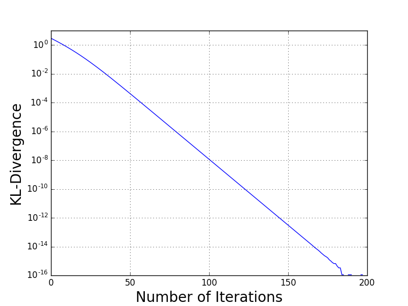Notice in particular the steady decrease of the KL-divergence to zero. The KL-divergence is only zero when the two distributions being compared are exactly the same; therefore, we see that the approximating distribution has converged to the target exactly.

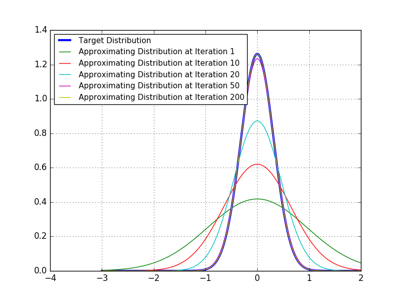
Second, we visually inspect the changes in the approximating distribution over time. Once again, we verify that the convergence to the desired target is achieved.

Future Directions

I am personally very excited about the applications of Stein variational gradient descent. I think it has great potential for learning parameters of Bayesian neural networks and other complex Bayesian systems; this is an important area of work in order for machine learning to harness well-calibrated uncertainties. In the next post in this series, we will be exploring the kernelized variant of Stein variational gradient descent, which is arguably more practically useful and powerful than the closed-form variety I demonstrated here.